One model to rule them all: Model convergence in CCAR, DFAST, CECL, IFRS9, and Basel, 3 Oct 2016

The Next Wave

First there was Basel II, with its subsequent years of interpretation, model development, review, documentation, and refinement. In retrospect, it's surprising how much effort went into estimating 12-month forward default rates under an average economy scenario.

Then came stress testing. CCAR (Comprehensive Capital Analysis and Review) and DFAST (Dodd-Frank Act Stress Testing) required banks to look further into the future (9 quarters) under alternate economic scenarios. This is a fundamentally more challenging task than Basel II, because one must quantify and incorporate economic sensitivities, adjust for attrition / pay-off, and quantify not just the probability of default, but also the timing of default.

As always happens with new regulations, lenders and regulators both evolve their knowledge and expectations of what should be considered standard practice. For CCAR, lenders consistently report that the Federal Reserve examiners want the best possible models and at the loan-level.

However, for the banks with assets less than $50 billion but greater than $10 billion that must only comply with DFAST, OCC and FDIC examiners are reported to have made comments such as, "If you build a more complex model, you will receive increased scrutiny." Thus, the path of least resistance for banks is to create simple time series models, even though such models fail to capture key portfolio dynamics and do not prepare banks for crossing the CCAR threshold.

Now we have CECL (the Financial Accounting Standards Board's rules for Current Expected Credit Loss) and IFRS9 (the International Accounting Standards Board's rules for International Financial Reporting Standards, latest revision), and both banks and examiners are groaning. Please, not another parallel model with different requirements and another cycle of interpretation, development, review, documentation, and refinement!

A Quick Review

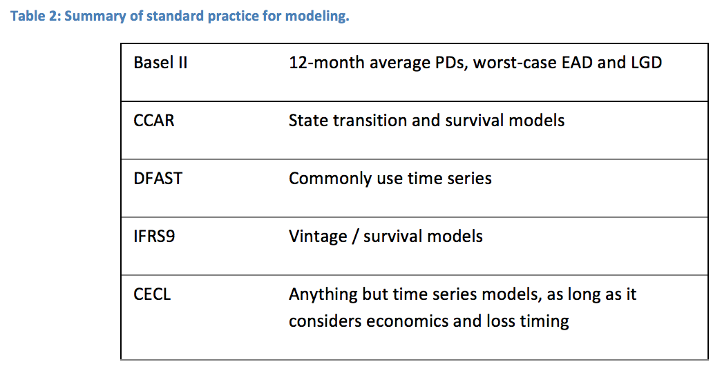
The following sections provide a quick review of common modeling practices for the different regulations. We will start with what is, before we look to what could be.

Base II

Although subsequent rules have been adopted to add to the initial calculation, Basel II continues to encapsulate the methodology for computing regulatory capital. Measuring regulatory capital is an exercise in quantifying the unknowable. We cannot know what a 1-in-a-thousand-year event looks like, but we know how that calculation should scale with the risk of the borrower and across products. Starting from some additional assumptions, Basel II provides a formula for the distribution of possible losses that can be scaled with a few input parameters. The task for lenders is to compute the probability of default (PD) for the next 12 months as an input to the formula.

The PD calculation is intended to be a through-the-cycle PD, meaning that it corresponds to the expected performance of the current portfolio in an "average" economic environment. Initial efforts took this to mean that an average of historic PD levels for the portfolio would be sufficient, but this failed dramatically because of the changing credit risk profile of loan portfolios through the economic cycle. Today, best practice is to make a forecast of the next 12 month PD for the specific loans on the books today, compensating for recent performance, age of the loans, and a scenario for an average economic environment.

Notably, Basel II does not require a forecast of when the future losses will occur, only the cumulative risk. Therefore, Basel II PD models tend to look more like traditional scores without adjustment for attrition or loss timing.

CCAR

In the 2009 Global Financial Crisis and concurrent US Mortgage Crisis, we must admit that Basel II did not perform very well. Either that or accept that 2009 was worse than a once-in-a-thousand year event. Unlikely.

CCAR is a direct response to the short-comings of Basel II. One OCC senior analyst gave a presentation where he demonstrated that the Basel II formula did not come close to fitting the in-sample data. His concluding remark for his talk was, "Don't trust the formula. Don't trust the result." Rather than employing a specific formula for which we know the starting assumptions are not met, at least for retail loans, banks are instructed to build their own models to predict portfolio performance under a specific set of macroeconomic scenarios.

Because CCAR models must incorporate specific macroeconomic scenarios and predict 27 months into the future, two things immediately change relative to Basel II. The forecasts must be time series and the models must capture the competing risks of default and attrition / pay-off. This means that CCAR models are not scores. We must start from a time series perspective, but they cannot be simple time series models either. Particularly for retail loans and deposits, the changing risk with the age of the loan can confound simple time series models. In other words, a simple time series model will only work if the portfolio is static in all respects other than macroeconomic drivers. It must be static in terms of the credit risk of new loans, the loan inflow volume must match the outflow, and the portfolio must be practically unmanaged in any sense that out impact account performance. None of these are ever true for any real-life portfolio.

Therefore, more sophisticated models have evolved as standard CCAR practice. The following table shows the primary model types that can satisfy the demands of CCAR stress testing. CCAR makes no explicit requirement for loan-level modeling, and past experience has shown that vintage aggregate models like Age-Period-Cohort (APC) models are very effective at long-range forecasting and stress testing. Roll rate models traditionally were use with simple moving averages of the rates, but roll rates are really just a structure. Those rates can each be modeled with more sophisticated methods, like vintage models.

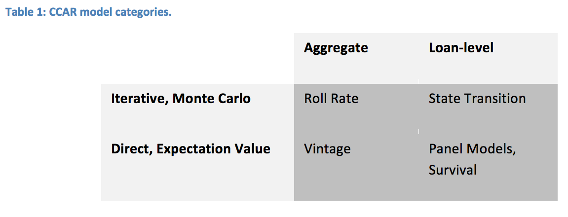
Although vintage aggregate models have been shown to perform well in the long run, they will be weaker than loan-level models in the first six months because of the inability to incorporate recent delinquency information. However, beyond this initial period, loan-level models have not shown any forecasting advantage over aggregate models, because any currently distressed account either defaults or cures beyond that point.

Nevertheless, CCAR examiners have expressed a clear preference for loan-level models. In this category, two model types have emerged as best practice. State transition models are just another name for Markov models. The states can be risk grades, delinquency buckets, or anything else where a given account can be described as having a unique state membership in a given month. To achieve long-range accuracy, the transitions need to depend upon economic factors, account performance factors, and the age of the loan. Terminal states should include charge-off and attrition / pay-off at a minimum. Although some of these transitions may be sparse or unmodelable, overall this type of model is usually created with multinomial regression to include a competing risk structure.

Forecasts with such state transition models are typically created via Monte Carlo simulation. At each time step, each account is randomly assigned to one of the states according to the predicted transition probabilities until the end of the forecast horizon is reached.

The last major model category is loan-level survival models. These include primarily Cox proportional hazards models or panel data models either with APC inputs for lifecycle and environment or in-place estimation of these effects. In all cases, macroeconomic factors and account performance factors can be incorporated along with the obvious lifecycle (hazard) function versus the age of the account. These models fit naturally with a competing risks framework, but usually simplify the problem to exclude modeling intermediate steps and focus instead on the end states. Forecasts are a simple loan-level expectation value of conditional probabilities of charge-off or attrition / pay-off at each month in the forecast horizon.

The best practice for these models is to make the model coefficients a function of forecast horizon, because the dependence upon delinquency-related measures will be highly dynamic over the first six months. By the time the twelfth forecast model is reached, the coefficients will have settled onto constant values for the rest of the forecast. This is equivalent to the convergence to steady-state seen in state transition models around the same horizon.

With sufficient data and careful treatment of multicolinearity among the factors, state transition and survival models actually become indistinguishable other than the choice of simulation versus expectation. Fortunately, state transition and survival models are known technologies. Enhancements will continue to be made, but either type can be used today to obtain universal applicability, so long as the validators, examiners, and auditors are prepared to accept them.

DFAST

For the smaller but still significant lenders, DFAST is the minimum stress testing requirement. The task for the modeler is no different from CCAR, i.e. build a long-range loss forecasting model that incorporates the same macroeconomic scenarios as CCAR. At this lowest level, none of the requirements have changed, so we would expect that DFAST models would be the same as CCAR models. However, with the intent of making things easier for smaller institutions, DFAST examiners have not pushed for the same model sophistication as CCAR examiners from the Federal Reserve. In fact, quite the opposite occurs.

Note that in the CCAR matrix, simple time series models were not shown. Modeling a default rate time series just with macroeconomic factors implies that everything else in the portfolio is steady-state. A steady-state portfolio is one for which new origination volume equals loan attrition / pay-off, origination credit quality remains constant, and management refrains from making any policy changes that would affect account performance. In practice, none of these are true. Therefore, simple time series models fail by design to capture the intrinsic dynamics of the portfolio and instead usually explain all historic performance changes with external macroeconomic factors -- Overfitting by design.

Where lenders move beyond simple time series methods, the preferred approaches will be the same as those described for CCAR, though probably with less emphasis on loan-level modeling.

IFRS9

IFRS9 is the new international accounting standard for estimating loan loss reserves. Unlike previous standards, IFRS9 requires a forward-looking estimate of losses. How the losses are estimated depends upon the performance of the loan. Three stages are recognized as shown below.

Stage 1: Performing loans - 12-month loss forecast
Stage 2: Significantly increased risk and not low risk - Lifetime loss forecast
Stage 3: Impaired loans - Lifetime loss forecast

For loans that are performing within tolerance of the original expectation (Stage 1), loss reserves are set at expected cumulative losses for the following 12-month period. This forecast should use a plausible economic scenario or a weighted average of a range of possible scenarios.

Loans that have exhibited significantly increased risk and are not considered low risk must have loss reserves set at the expected cumulative lifetime losses. No fixed criteria are available for movement to Stage 2. Some may set the threshold as a predetermined level of delinquency. Others may set a specific score or PD threshold to determine the threshold. For the lifetime forecast, a plausible economic scenario for the first 12 months should relax onto a long-run average for the remainder of the lifetime forecast. Again, a weighted average of multiple scenarios may be considered best practice.

Impaired loans are classified as Stage 3. At this stage, interest revenue recognition changes to a net interest basis, but the loss estimation remains the same as in Stage 2.

One could naturally perform all of the above analysis at the loan-level, making individual assessments of increased credit risk. However, the IFRS9 guidelines specifically state that pooled analysis may be necessary to identify the increased risk of an individual loan. As seen in the US Mortgage Crisis¹, an account may be in a vintage and segment that is experiencing much higher than expected losses. Although that account may not be exhibiting stress, through membership in that specific vintage / segment the account may warrant Stage 2 loss estimation.

Because of this support of pooled analysis and the need for lifetime loss estimation from any account age through to the end of term or foreseeable future, vintage models have rapidly become the standard for IFRS9 loss estimation. In Europe, the standard approach is referred to as EMV modeling (Exogenous-Maturation-Vintage). EMV models are a direct derivative of the vintage decomposition method called Dual-time Dynamics which is in turn largely equivalent to Age-Period-Cohort models. All these vintage analysis methods decompose the historic performance into functions of age, vintage, and time.

¹ Reference to our mortgage article.

With such vintage analysis models, for Stage 1 the first 12-months of the forecast under a baseline economic scenario can be aggregated as the loss forecast for all vintages that are within a predefined range of average risk. For Stage 2, the high-risk vintages within risky segments will have their loss forecast set to the cumulative loss over the life of the loan under a through-the-cycle economic scenario for the period beyond the first year.

Because the vintage risk estimates stabilize within a year of origination, this approach has the advantage of being relatively stable. Risky vintages will likely maintain that designation for the life of the loan.

Loan-level modeling is an attractive option for IFRS9 because of the intuitive desire to isolate those accounts that are causing the increased risk. However, since the IFRS9 guidelines specifically comment on the need to set higher reserves even for accounts that do not currently show risk but are associated with other accounts that do, we need a definition for Stage 2 that is more expansive that something like delinquency.

For a loan-level definition of Stage 2 increased risk, looking beyond delinquency we could also consider utilization (for lines-of-credit), credit bureau scores, debt-to-income, loan-to-value (for auto or mortgage), etc. Therefore, a loan-level model can be created to incorporate these factors, but it must also incorporate lifecycle effects in order to provide lifetime loss estimates, economic factors, and residual vintage risk beyond the score. Also, we need to capture the attrition probability so that the lifetime estimates are correct.

The above can be achieved with Cox proportional hazards models or a scoring model that takes lifecycle and environment as inputs. The loan-level model would not need to be used for the Stage 1 loss forecast, but only to assess when the loan's credit risk has exceeded a predetermined bound. Then the loan-level model could be used to assess the lifetime loss.

State transition models can also be used to fulfill the needs of IFRS9. Although in practice they tend not to strongly model the lifecycle effect, this can be incorporated in most cases. One caveat is that the Stage 2 and Stage 1 models should be closely connected so that the estimates, though different because of the different forecast horizons, are still consistent.

CECL

CECL was developed concurrently with IFRS9, but elected to use lifetime loss estimation for all loans rather than having a multi-stage approach. This decision was to simplify the process for the thousands of small lenders in the US. The stated goals of lifetime loss estimation and using current economic conditions for the near-term and relaxing onto the long-run economic conditions for the rest of the forecast naturally lead to the same kind of models discussed above for IFRS9. However, in an attempt to soften the burden for smaller institutions, the CECL guidelines state explicitly that complex models are not required by smaller institutions. Nevertheless, finding a simpler approach that does not carry a harsh penalty in loss reserve levels or in auditor and examiner review is not obvious.

CECL and IFRS9 modeling needs actually come closest to CCAR. Lenders of all sizes and business models, if they want models that are defendable to auditors and examiners, will need models with economic sensitivity, competing risks of attrition and default, and monthly or quarterly forecasting through the life of the loan. The best models will be loan-level so that they consider current loan conditions and integrate with accounting systems.

Comparing Regulations

How do we bring unity to such differing requirements? With a few nudges, it's quite possible. Basel II and DFAST are the outliers. If we start from Basel models, the gap to CCAR or CECL / IFRS9 is quite wide. A 12-month average Basel PD could be viewed as an input to a more complete model, but the simplest approach is to start from CCAR or CECL / IFRS9. A best-in-class CCAR model would provide loan-level, monthly default rate forecasts with adjustment for attrition and economic scenarios. To satisfy Basel, one need only use a through-the-cycle economic scenario and aggregate the first 12-months of the forecast.

Clearly, a large bank building a CCAR-compliant model can use the same model for DFAST, but if we start from one of those commonly-built DFAST time series models, life is not easy. A simple time series model will not work for CECL or IFRS9, because it does not capture any lifetime loss aspects. In fact, it's not even clear how it can comply with DFAST given how much of the portfolio's key dynamics are lost, but so far they have been accepted. For DFAST lenders that are not large enough for CCAR, satisfying CECL or IFRS9 may push them to create CCAR-class models anyway, and their DFAST submissions will be much better because of it. Thinking through the similarities and differences between all these requirements leads us to the follow commonalities.

Economic sensitivity (to model different economic scenarios)
Monthly or quarterly forecasting (to incorporate economic scenarios)
Competing risks of default and attrition / pay-off (for long-range forecasting)
Lifecycles in loss and attrition / pay-off timing (for long-range forecasting)
Loan-level (for CCAR and best-practice CECL / IFRS9 and Basel)

In most general terms, two primary classes of model can satisfy these needs: state transition models and survival models.

For decades, lending analytics were little more than credit scores and moving average roll rate models, but neither of these methods was forward-looking. Notable, all mortgage lenders prior to the US Mortgage Crisis had both roll rates and credit scores. Of course, few claim to have predicted the collapse in house prices, but the increased default rates due to higher risk loans and the timing of those losses were quite predictable. In fact, simple vintage models performed quite well through the mortgage crisis. With the failure of moving average methods made blatantly clear, all areas of regulation are moving to forward-looking methods.

Although the transition can be painful, one wonders how we can function without these. How can loans be priced without knowing the expected lifetime losses? If profits are large and competitors are few, then portfolio management can be passive and models are not necessary. That environment has not existed in lending since about the 1980's. To survive today, these models are needed throughout the organization. Model convergence is just making sure the we create good models across the range.

Prev Blog Next