Santa Fe, NM 87505
CECL Procyclicality: It Depends on the Model, 14 Sep 2018
The new guidelines for loan loss reserves, CECL (Current Expected Credit Loss), were initially proposed so that lenders' loss reserves would be forward-looking. Some recent studies have suggested that CECL could be procyclical, meaning that loss reserves would peak at the peak of a crisis. Although better than seeing failure only after it has happened, being required to raise liquidity at the peak of a crisis could still fail to save the lender from collapse, or even facilitate it.
However, previous procyclicality studies explained all losses with macroeconomic factors, ignoring the changes in credit risk and other portfolio drivers that preceded the recession. The current work tests a wide range of models to test the degree to which CECL is procyclical for different types of models. The tests were also run using either real historical macroeconomic scenarios , flat scenarios, or mean reverting scenarios. All tests were conducted on publicly available data from Fannie Mae and Freddie Mac using publicly disclosed models.
This study found that the CECL lifetime loss estimates were only marginally sensitive to the quality of the economic scenario but changed dramatically with different modeling techniques. Some methods predicted increased loss reserve requirements as early as 2006 while others only saw the recession as it happened or even afterward. Therefore, procyclicality under CECL will be strongly influenced by the choices of the lender.
Keywords: Current expected credit loss approach, loan loss provisions, procyclicality, vintage models, roll rate models, state transition models, survival models
JEL Classifications: G18, G21, G28,
1 Introduction
Following the 2009 US recession and global financial crisis (GFC), the FASB (Financial Accounting Standards Board) and IASB (International Accounting Standards Board) sought new loan loss reserve rules that would allow lenders to reserve for losses that could be reasonably anticipated given what is knowable in their portfolio and the economy. This was intended as an improvement over the previous rules which were inherently backward looking, considering only losses after a default was believed to have occurred. Furthermore to this goal, loss reserves were to look further into the future. In the US, the new rules adopted in June 2016, the current expected credit loss (CECL), set all loss reserves to cover the full lifetime of the loan [15]. The international standard, IFRS 9, uses a 12-month loss reserve for stage 1 accounts (performing as expected), but also adopts a lifetime loss calculation for stage 2 accounts (increased risk) [23]. The primary motivation for the divergence in the standards was the need to accommodate the thousands of smaller lenders in the US. Therefore, CECL is essentially IFRS 9 stage 2 for everyone.
Given the goal of anticipating and reserving for future loss events, the 2009 US recession and GFC serve as good test cases of whether loss reserves under these rules would lead, lag, or be coincidence with the crisis. Although provisions that lag the crisis serve little purpose, as was true under the old rules, provision requirements that peak coincident with the crisis can also cause significant financial stress because of the difficulty raising capital during a crisis. When loss provision requirements are coincident with the underlying losses, this is referred to as procylicality.
To prepare for future macroeconomic stresses, we should determine how we can reasonably expect CECL estimates to behave. By applying CECL to the 2009 US recession in the case of mortgage and considering what was knowable at the time, we seek to determine the degree to which CECL would be procyclical. Most importantly, prior experience has shown that different modeling approaches can provide different degrees of foresight, so we tested time series, vintage, roll rate, state transition, and survival models, all of which are statistical techniques. In addition, we considered some simple, spreadsheet-based methods that have been recently proposed for use by smaller organizations to comply with CECL. These are loss timing, vintage copy forward, and weighted average remaining maturity (WARM).
To capture what was knowable at each forecast point, we purchased historic publications of macroeconomic scenarios from Consensus Economics corresponding to the month before each forecast date. Those scenarios were for the following two years. Using that as the "foreseeable" period, we applied a mean-reverting algorithm to the scenarios in order to forecast the remainder of the term of the 30-year fixed rate conforming mortgages from Fannie Mae and Freddie Mac. We also considered a flat macroeconomic extrapolation for two years followed by mean reversion. The third option was immediate mean reversion. Any of these approaches would have been realizable through the economic cycle.
The results of this study show the extreme importance of which model is cho- sen for CECL. Also, once we abandon perfect foresight, the differences between realistic economic scenarios are minor.
This study was inspired by the results of previous studies. An early study on procyclicality argued on largely theoretical grounds that CECL would reduce procyclicality [10]. However, these conclusions made several assumptions about what lenders would be able to estimate. A more recent analysis showed that CECL estimates for mortgage would have been countercyclical if the future macroeconomic conditions were known [9]. Neither of these studies addressed the question of the real-world timing of CECL provisions given what was knowable at the time.
Most recently, a study by Covas and Nelson [11] created a vector autoregression model to generate macroeconomic scenarios at each forecast point. These were fed into a time series model similar to what is included in the current work. Their result was that CECL estimates are highly procyclical and would have caused a worsening of the crisis through reduced liquidity and subsequent lending by banks. Their study did not consider any other model types.
In fact, previously published work on the mortgage crisis has shown that losses did not peak purely due to deterioration in the economic environment. Several authors have explored the impact of the moral hazard of securitization as driving risky lending [13, 28, 30]. Levitin, Pavlov, and Wachter [29] argued that securitization was the sole cause of the crisis, although this is rebutted by Foote, Gerardi, and Willen [18].
Breeden [5] used a dataset back to 1990 to identify credit cycle peaks in 1991, 1995, and 2001 to argue that although securitization played a deleterious roll in the 2009 crisis, this loss peak also corresponded to a credit risk cycle. A subsequent analysis by Breeden and Canals-Cerda used a richer, more recent data set to show that half of the mortgage crisis was explainable by typical scoring factors. Although some part of the residual could have been attributable to unseen underwriting changes, it again correlates strongly to drivers of consumer risk appetite as measurable from the FRB Senior Loan Officer Opinion Survey (SLOOS).
Regardless of the exact mix of effects identified by these authors, the message from all of them is that mortgage losses were more than an economic crisis. One could assume that economic crises are unpredictable, but credit cycles are a different matter. This leaves the possibility that losses are not as unpredictable as some have assumed, if the correct model is used.
2 Data
This test was performed on publicly available data from Fannie Mae and Freddie Mac. Specifically, 30-year conforming fixed rate mortgages were analyzed. Loan- level information from 2001 through 2017 from both sources was normalized and combined. In addition to monthly loan status, the database contains a number of attributes suitable for loan-level credit risk estimation. The full list of data fields for Fannie Mae and Freddie Mac appears in Table 1.
For the models developed in the study, the following definitions were used:
- Default: current loan delinquency status >= 3, i.e. 90+ days past due (DPD)
| Origination fields | Performance fields |
|---|---|
| Loan sequence number | Loan sequence number |
| Credit score | Monthly reporting period |
| First payment date | Current actual UPB |
| First time homebuyer flag | Current loan delinquency status |
| Maturity date | Loan age |
| Metropolitan statistical area | Remaining months to legal maturity |
| Mortgage insurance percentage | Repurchase flag |
| Number of units | Modification flag |
| Occupancy status | Zero balance code |
| CLTV - cumulative loan to value | Zero balance effective date |
| DTI - debt to income | Current interest rate |
| Original UPB (unpaid balance) | Current deferred UPB |
| LTV - loan to value | DOLPI - Date of last paid installment |
| Original interest rate | Mortgage insurance (MI) recoveries |
| Channel | Net sales proceeds |
| PPM flag | Non MI recoveries |
| Product type | Expenses |
| Property state | |
| Property type | |
| Postal code | |
| Loan purpose | |
| Original loan term | |
| Number of borrowers | |
| Seller name | |
| Servicer name |
Table 1: Origination and performance data fields available in the Fannie Mae and Freddie Mac datasets.
- Active: non-default and current actual UPB> 0
- Attrition: zero balance code=1 (prepaid)
- Outstanding balance: current actual UPB if status = Active
- Default balance: current actual UPB if status = default
- Origination balance: current actual UPB if Current Date = Vintage
- Loss: Default balance + Accrued Interest + Total Costs Total Proceeds
- Accrued interest: Default balance*((Current Interest Rate/ 100-0.0035)/12)*(Months between Last Principal and Interest Paid Date and Zero Balance Date)
- Total costs: Foreclosure Costs + Property Preservation and Repair Costs + Asset Recovery Costs + Miscellaneous Holding Expenses and Credits + Associated Taxes for Holding Property
- Total proceeds: Net Sales Proceeds + Credit Enhancement Proceeds + Repurchase Make Whole Proceeds + Other Foreclosure Proceeds
The data analyzed in this study represents more than $2 trillion of conforming mortgages. All models were segmented by risk grade: Subprime is less than 660 FICO, Prime is 660 to 780, and Superprime is 780 and above. Although data was available by zip code, only nationwide models were created in alignment with the available macroeconomic scenarios.
2.1 Macroeconomic Scenarios
The macroeconomic scenarios in this study were obtained by purchasing reports from Consensus Economics published in the month preceding each quarter’s forecast, so these CECL estimates use the real economic assumptions available at the time. Consensus Economics provides quarterly scenarios for the following two year period. From the factors provided, the following were considered for mortgage modeling: real gross domestic product, real disposable personal income, unemployment rate, 3-month treasury bill rate, and 10 year treasury bond yield. These scenarios represent the average predictions of 24 prominent economists or economic forecasting institutions.
Figure 1 shows that the consensus economic scenarios follow a rational pattern. In any quarter, they follow recent trends and then begin to revert to loan run averages.
The models tested here were originally developed as part of a more extensive CECL mortgage study [7]. In that study, the selection of macroeconomic factors was chosen from mortgage-related factors that are available in the government’s Dodd-Frank Stress Test Act (DFAST) scenarios. in order to maintain reproducibility of the results, Among the factors considered in the models, house price index (HPI) and Dow Jones Total Stock Market Index were missing from the Consensus Economics list. The Dow Jones index rarely appears in the models, but HPI is quite important. To run the models, a simple vector auto-regression model was created to predict the values of the missing variables from the available data of all macroeconomic factors. This modeling was training on data preceding each forecast date. Accuracy was not a primary concern, only that the models could be run out-of-sample.
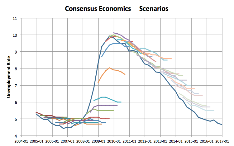
Figure 1: Quarterly unemployment rate scenarios from Consensus Economics Inc. for the following two years. A mean-reverting scenario is applied thereafter to complete the CECL forecast.
3 Models
CECL is built on models. To study procyclicality, the models developed in the CECL mortgage study by Breeden [7] were employed along with some recent additions: WARM, Vintage Copy-Forward, and Loss Timing. The following sections provide summary descriptions of each model. The complete descriptions are available in the original study details.
3.1 Time Series
The simplest forward-looking model in this study requires creating macroeconomic time series models of the balance default and pay-down rates. Lifetime losses can then be simulated by projecting forward under a mean-reverting base macroeconomic scenario until all currently outstanding balances are either paid or charged off. Transformation of the macroeconomic data and model estimation are primary considerations [26, 25, 14, 36, 20].
The time series model used macroeconomic factors to predict the balance loss rate and balance payment rate, segmented by subprime, prime, and super- prime. These models use lagged transforms of the economic factors described in Section 2.1.
Pure macroeconomic time series models necessarily assume that all portfolio dynamics are explainable by the economy without regard to changes in underwriting or other policies. As mentioned in the introduction, many other factors may have contributed to the mortgage crisis. In this time series model, those factors will either be absorbed indirectly via possibly spurious correlations to macroeconomic factors, or missed entirely.
3.2 Roll Rate
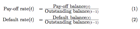
For the last 40 years, the two most common kinds of models for retail lending portfolios are credit scores and roll rates. Roll rate models are similar in spirit to a state transition model, but estimated on aggregate monthly balance flows from one delinquency bucket to the next. [16]
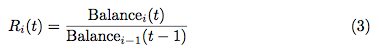
Historically roll rate models have used moving averages of past rolls. For CECL estimation, Ri(t) is modeled with macroeconomic factors. In addition, the balance pay-down rate for non-delinquent accounts is modeled with macroeconomic data so that both charge-off and pay-off end states are included. Thus, the roll rate model is like the time series model, but with intermediate delinquency transitions added. The final lifetime loss is calculated by summing the monthly losses until all existing loans reach zero balance.
3.3 Age-Period-Cohort (Vintage)
Vintage models naturally capture the timing of losses and attrition versus age of the loan, and therefore are an obvious choice for lifetime loss calculations. An Age-Period-Cohort approach is commonly used to estimate such models [19, 21, 4, 8]. Using rates for probability of default (PD), exposure at default (EAD), loss given default (LGD), and probability of attrition (PA), monthly loss forecasts are created and aggregated to a lifetime loss estimate.
When modeling default rate (PD), this takes the following form:
log-odds(PD) = lifecycle(age) + credit risk(vintage) + environment(date) (4)
Age is the age of the vintage. Vintage is the origination date. The lifecycle is also known as the hazard function or the loss timing function. Credit risk measures the relative risk of each vintage. Environment captures macroeconomic impacts and account management changes through time.
The lifecycle, environment, and vintage functions can be represented with splines or nonparametrically. The coefficients for those functions are typically estimated with logistic regression or with a Bayesian estimator [31]. To obtain a solution, a constraint must be set on the linear trends, as described in the APC literature [22].
Macroeconomic scenarios are used to project the future value of the environment function, which is then combined with the vintage and lifecycle functions to produce monthly forecasts for each vintage. The lifetime loss forecast sums across both vintages and calendar date to the end of the loans’ terms or until the outstanding balances reach zero.
3.4 State Transition
State transition models are the loan-level equivalent of roll rate models. Rather than modeling aggregate movements between delinquency states, the probability of transition is computed for each account. The states considered are current, delinquent up to a maximum of six months delinquent, charge-off, and pay-off. Account transition probabilities are modeled rather than the dollar transitions in the roll rate model.
They derive from Markov models, though in practice they may not satisfy the Markov criteria that no history other than the current state is used in the model. They were used first and most heavily for corporate ratings and commercial lending, where most of the literature is still to be found [24, 35, 33]. However, they are often used for retail lending, most often for mortgages [32, 2]. The method used here is most like that of Berteloot, et. al. [3].
For modeling, a recommended approach would be to create a multinomial regression model from each non-terminal state, predicting all of the other states the account can transition to. The regression model would consider external macroeconomic drivers as well as internal factors for the accounts, such as FICO, loan-to-value (LTV), etc. Functions of age may also be included in order to capture lifecycle effects.
To make forecasts, if the input variables to the transition probability models satisfy the Markov condition of having no memory prior to the current state, then the forecasts may be created via a series of matrix multiplies as in the Markov chain approach. However, if the input factors do have memory, such as number of times delinquent in the previous six months (a common predictive factor), then a Monte Carlo approach must be applied to a sample of the accounts to simulate possible portfolio performance. At each time step each account is assigned a specific state based upon the probability of that transition and a drawn random number.
In all cases the probabilities are functions of time, because the macroeconomic scenarios will change with time using the same mean-reverting scenarios described earlier. The accounts will be simulated until they reach a terminal state such as charge-off or pay-off, or they reach the end of term.
EAD and LGD are modeled separately as functions of the age of the loan to capture balance pay-down with time.
3.5 Multihorizon Discrete Time Survival Model
Conceptually, discrete time survival models are the loan-level enhancement to vintage models, usually with the implication of creating loan-level models with scoring attributes. They did not evolve from survival models, but the relationship is fair. Because lending performance data is generally recorded in monthly increments, the discrete time approach is appropriate, in which case a discrete time survival model is identical to logistic regression with a hazard function as a fixed input.
For the present study, the lifecycle and macroeconomic correlations from the APC vintage model estimation are used as fixed inputs to a logistic regression panel data model with scoring attributes. This two-step process is done to avoid multicolinearity problems when trying to estimate everything simultaneously. PD, PA, and EAD are estimated with this process.
Separate origination and behavioral models are built, the former using only factors available at origination and the latter using both origination factors and behavioral factors such as recent delinquency. The multihorizon aspect comes from the fact that a separate regression is estimated for each forecast horizon. This is done because the coefficients for delinquency are highly nonlinear with forecast horizon. However, by horizon 12, the coefficients stabilize and can be used for all future values. Because any delinquent account will have either cured or charged-off within six to twelve months, the remainder of the forecast is dominated by persistent factors like FICO score and LTV.
The final lifetime loss forecasts are created by aggregating the loan-level monthly loss estimates.
3.6 Weighted Average Remaining Maturity (WARM)
Popularized in FASB webinars on simple CECL approaches [17], WARM is just the multiplication of the recent average loss rate and the average expected life of the loan. Average expected life could be defined as the age at which half the loans have paid-off or charged-off, or it could be defined as the age at which the average outstanding balance will be half of the initial balance, which would be shorter than the former. If one were to multiply the loss rate by the outstanding balance in each month of the loan, adjusted for prepayment risk, the result would be equivalent to the age at which the outstanding balance is half of the initial balance. That is the approach used here.
Most notably with WARM, the loss rate used in the calculation is not dependent upon the age of the account, economic conditions, current delinquency or any credit risk factors. This is a steady-state model where all such changes are assumed to be introduced manually via quantitative adjustments (Q-factors).
3.7 Vintage Copy-Forward
One simple method proposed for complying with CECL is to apply the annual loss rate of the previous vintage in the previous year to the current vintage in the current year. This has the affect of aligning vintages by age and potentially capturing some recent credit quality changes.
To create the lifetime loss forecasts required by CECL, each successive forecast year must look to an older vintage. If credit quality is not a constant across vintages, this will create a bias in the approximation versus age. Also, this approach does not include any explicit macroeconomic correlations.
3.8 Loss Timing
Lastly, the loss timing approach is conceptually the same as a balance-based hazard function [12], but computed simply in a spreadsheet as the average monthly loss rate versus age of the vintage. The vintages are aligned by age and an average balance loss rate is computed relative to the origination balance. To create forecasts, the loss timing function is applied for all forecast horizons for active vintages.
Because this is a simple spreadsheet average rather than a statistical estimate of a hazard function [27, 1], it will be subject to a number of biases. Again, this is being proposed as a CECL solution, but would not normally be considered a model suitable for forecasting.
4 Results
The goal of the study is to simulate how these models might perform out-of- sample. To achieve that, one would ideally estimate all of the coefficients only on data prior to the start of each quarter’s forecast. The challenge is that this data does not have enough history prior to the recession to fully estimate these models. Further, when we apply these models to the next recession, we will have this past recession to model against. Although no future recession is expected to be a replay of the previous recession, having one to train on is better than no historic data.
With all this in mind, it would be overly harsh to run the models with no history, and yet we don’t want to give perfect foresight. The compromise used is that the full history was used to estimate economic sensitivity and product lifecycles, but not scoring coefficients. It has been the author’s personal experience that lifecycles for a specific product like 30-year mortgage are stable through time and across lenders.
Macroeconomic sensitivities, when the correlations are restricted to variables close to the consumers’ finances, are also reasonably stable. Unemployment and change in house prices are always the dominant effects for mortgages. The biggest change between the 2009 recession and the 2001 recession was the lengthening of unemployment benefits to 99 weeks. This was significantly greater than previous recessions and appears to have caused the optimal lag between unemployment and mortgage default to have increased.
For the time series and roll rate models, estimating macroeconomic factors across the full data set means that they are fully in-sample. For all other models, the macroeconomic sensitivities were taken from a model over the full data and other coefficients were re-estimated each quarter using only the preceding data. As will be seen later in the scenario comparison results, using partially out-of- sample models probably makes no difference in the comparison.
4.1 Comparing Models
The models described above were run each quarter using the corresponding macroeconomic scenario as illustrated in Figure 1 for the first 24 months. Then a mean-reverting algorithm was applied to the optimally transformed macroeconomic factors using a second order Ornstein-Uhlenbeck algorithm [34, 6]. Each point along the time series in Figure 2 represents the CECL lifetime loss estimate at that point for the Fannie Mae / Freddie Mac mortgage portfolio. A CECL estimate was run for each quarter from 2005 Q1 through 2015 Q4.
The black line in Figure 2 is the actual future lifetime loss for loans outstanding at that forecast point. The actual performance data runs through 2017, so the tail losses beyond 2017 were filled in with a vintage model, because that was one of the most accurate in our previous study. The actual forward-looking lifetime losses rise steadily between 2005 and mid-2008, because new higher-risk loans were being originated at a rapid pace.
The Actual line is an unobtainable ideal, but at the far opposite extreme is the light green line for WARM. The graph shows that WARM is really no different from the moving average loss rate typically used previously for ALLL calculations, just with a lifetime multiplier. As such, it peaks well after the crisis is over at a time that all other models correctly predict decreasing loss reserves. Regulatory expectation is that users would apply quantitative factors (Q-factors) to manually adjust the WARM baseline to expectations about the economic and credit cycles. However, because WARM is so out-of-phase with actual reserve needs, lenders would be better off using a completely flat (through-the-cycle) average loss rate than to try to back out the post-peak behavior of WARM. In short, WARM should not be used for CECL.
Between these extremes of perfect foresight and pure hindsight, things get much more interesting. The most important question is not when reserves will peak. In any recession scenario, reserves will peak when the macroeconomic peak is known. However, not all losses are driven by macroeconomic factors. When large volumes of new loans are booked, the hazard function or APC lifecycle will predict when those losses should occur in the future. Similarly, a strong credit cycle exists in mortgage, which can also be incorporated in the forecast. Therefore, the question is whether any of the models give a warning or simply jump to peak levels at the last moment. Figure 3 shows the change in quarterly CECL estimates as a percentage of the outstanding loan balance.
The time series model that other studies suggest would be procyclical is, in fact, procyclical. Loss reserves do not begin to rise until late 2008. In the period between 2005 and late 2008 when large volumes of risky loans were being booked, the time series model shows no increase in reserves. If this were the only basis upon which CECL was judged, it would be considered a failure. However, that is a failure of the model, not the guidance.

Figure 2: CECL lifetime loss estimates between 2005 and 2015 for a range of models using Consensus Economics scenarios the month before the forecast quarter.
The best two models from the perspective of anticipating the crisis are the Age-Period-Cohort (vintage) model and the multihorizon discrete time survival model. Both the APC and survival models start increasing reserve estimates in 2005 and accelerate provisioning through 2009. Notably, these models are adding reserves when the consensus economic scenario suggests that nothing is wrong economically. Rather, the models are responding to shifts in credit quality and applying the loss timing to the new originations. Although only halfway to the perfect foresight result, they would have provided an early warning to lenders as early as 2006 that risks were increasing significantly. This should be the stated goal of CECL not to predict the economic cycle, which is unlikely, but to accurately forecast the risk already in the portfolio.
The roll rate is better than nothing, but only halfway to the vintage and survival models. This roll rate model used time series models of the net roll rates to incorporate the economic cycle. A more simplistic model that only uses moving averages of the rolls, as is common practice, would give much less warning.
Also shown is the state transition model. As seen in Figure 2, the state transition model showed rather little response to the recession. Unlike the roll rate model which fits directly to the economic cycle, the state transition predicts only one step ahead (one month). Therefore, it’s coefficients are optimized for short term accuracy, not accuracy through the economic cycle.
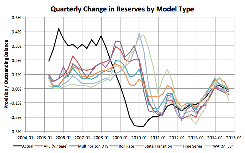
Figure 3: Change in quarterly reserves by each model type using the Consensus Economics scenarios.
Table 2 summarizes the change in CECL reserves as estimated by each model. The values shown are as a fraction of the ideal reserve level that would have been maintained with perfect foresight. The results are ranked by which models gave the most advance warning during the critical period of 2005 through 2007.
The results in Figure 3 and Table 2 are not the actual quarterly provisions required, because provisions also must include replacement of charge-off expenses in the previous quarter, Equation 6.
Provisions(t) = Reserves(t) − Reserves(t − 1) + Losses(t − 1) (6)
Figure 4 shows the quarterly provisions that would be required under each model as a percentage of outstanding balances in that quarter. Comparing provisions makes the models look more similar, because they all add in the replacement of charge-off balances, even when the CECL calculation is unchanged.
We distinguish here between a statistically-based vintage model and some simplistic spreadsheet-based vintage models, because the latter are in the same league as WARM and serve only to clutter the earlier graphs. Figure 5 shows the reserves for the other spreadsheet-based methods in context of a few statistical methods. Of these, the Loss Timing model comes the closest to providing a stable baseline against which to add intuitive Q-factors by management. The Vintage Copy-Forward and
WARM methods are essentially unusable.| Model | 2005-2007 | 2005-2008 | 2005-2009 |
|---|---|---|---|
| APC (Vintage) | 42.0% | 52.7% | 82.9% |
| Multihorizon DTS | 36.3% | 48.1% | 83.8% |
| State Transition | 28.3% | 35.0% | 47.9% |
| Roll Rate | 24.3% | 31.4% | 49.3% |
| Vintage Copy-Forward | 18.9% | 69.4% | 231.1% |
| Time Series | 13.5% | 17.2% | 38.6% |
| WARM, 5yr | 5.3% | 12.3% | 35.4% |
| Loss Timing | 0.9% | 1.3% | 0.3% |
Table 2: Changes in quarterly CECL estimates as a percentage of outstanding balance.
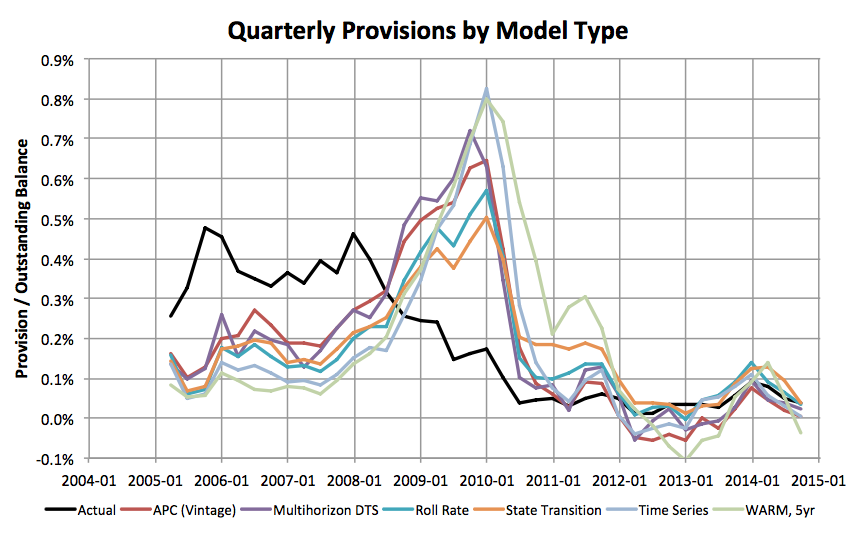
Figure 4: Quarterly provisions required by each model type using the Consensus Economics scenarios.
That fact that APC, Loss Timing, and Vintage Copy-Forward are all "vintage" models has greatly confused the discussions around how to implement CECL. Clearly, not all vintage models are the same.

Figure 5: CECL lifetime loss estimates between 2005 and 2015 for the spreadsheet models compared to some key statistical methods using Consensus Economics scenarios the month before the forecast quarter.
4.2 Comparing Scenarios
In the preceding analysis, we used real macroeconomic scenarios from the forecast periods, but how important is it to obtain the best possible scenarios? Figure 6 shows the sensitivity of the APC CECL estimates to macroeconomic scenarios. The blue line is the forecast with perfect foresight for the full life of the loans. The red line uses perfect foresight for the first two years, but then applies a mean-reverting algorithm for the remainder of the forecast. Therefore, the red line is the best possible CECL estimate, because it complies with the CECL rules about reverting to long-run averages beyond a ”reasonable and supportable” period. The two-year reasonable and supportable period used here appears to be the most common value chosen in the industry.
The other lines use either consensus, flat, or mean reverting for the first two years, and then continue with mean reverting for the remaining life of the loan. Other than the Actual and Actual, 2yr scenarios, all other scenarios are plausible CECL approaches.
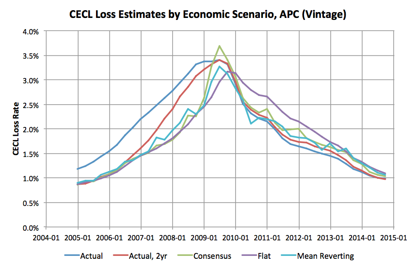
Figure 6: CECL lifetime loss estimates using various macroeconomic scenarios in the APC vintage model.
Until January 2007, the Actual, 2yr and all realistic scenarios are equivalent. All of the realistic scenarios diverge from perfect foresight between January 2007 and January 2009. However, all of the realistic scenarios are roughly equivalent during this period and provide the early warning shown in Figure 3, because that early warning is not dependent upon economic cycle. The consensus economic scenario is more accurate and one quarter earlier than the flat scenario, but the difference is minor. This result suggests that creating a good forecasting model is more important than finding an optimal macroeconomic scenario.
5 Conclusion
During the initial adoption phase for CECL, the biggest step for lenders will be to establish appropriate risk management practices for loss reserves, gather necessary data, and create the necessary systems. During this time, any model will probably be acceptable so long as overall progress is shown.
However, the purpose of CECL is to help lenders survive crises. Simple models appear to offer little help in surviving crises and may actually be harmful. To be useful in the period leading up to a crisis, having an effective model will be important.
The current results also demonstrate that the model is more important than the economic scenario. We accept that perfect macroeconomic foresight would be useful, but is unobtainable. After that, the difference between the best and the worst realistic macroeconomic scenarios is slight, but the difference between the best and worst models is dramatic.
Acknowledgements
The author wishes to thank Maxim Vaskouski for his assistance in conducting tests for this paper.
Also, Deep Future Analytics LLC (www.deepfutureanalytics.com) was an important sponsor of this work.
References
[1] O. Aalen. Nonparametric inference for a family of counting processes. Annals of Statistics, 6:701–726, 1978.[2] A. Bangia, F. X. Diebold, A. Kronimus, C. Schagen, and T. Schuermann. Ratings migration and the business cycle, with application to credit portfolio stress testing. Journal of Banking & Finance, 26(2):445 – 474, 2002.
[3] K. Berteloot, W. Verbeke, G. Castermans, T. V. Gestel, D. Martens, and B. Baesens. A novel credit rating migration approach using macroeconomic indicators. Journal of Forecasting, 32:654–672, 2013.
[4] J. L. Breeden. Modeling data with multiple time dimensions. Computational Statistics & Data Analysis, 51:4761 – 4785, May 17 2007.
[5] J. L. Breeden. Macroeconomic adverse selection: How consumer demand drives credit quality. In Credit Scoring and Credit Control XII Conference, Edinburgh, August 2011.
[6] J. L. Breeden. Living with CECL: Mortgage Alternatives Study, chapter 10. Mean-Reverting Scenarios. Prescient Publshing, 2018.
[7] J. L. Breeden. Living with CECL: Mortgage Modeling Alternatives. Prescient Models LLC, 2018.
[8] J. L. Breeden and L. C. Thomas. The relationship between default and economic cycle for retail portfolios across countries: identifying the drivers of economic downturn. Journal of Risk Model Validation, 2(3):11 – 44, 2008.
[9] S. Chae, R. Sarama, C. Vojtech, and J. Wang. The impact of the current expected credit loss standard (cecl) on the timing and comparability of reserves. Technical report, Bank Policy Institute, 2018.
[10] B. Cohen and G. Edwards. The new era of expected credit loss provisioning. Technical report, Bank for International Settlements, March 2017.
[11] F. Covas and W. Nelson. Current expected credit loss: Lessons from 2007- 2009. Technical report, Bank Policy Institute, July 2018.
[12] D. R. Cox and D. O. Oakes. Analysis of Survival Data. Chapman and Hall, London, 1984.
[13] R. Elul. Securitization and mortgage default. Journal of Financial Services Research, 49:281– 309, 2015.
[14] W. Enders. Applied Econometric Time Series, Second Edition. John Wiley & Sons, 2004.
[15] FASB. Financial Instruments Credit Losses (Subtopic 825-15). Financial Accounting Series, December 20 2012.
[16] FDIC. Credit card activities manual. https://www.fdic.gov/regulations/examinations/credit card/ch12.html, 2007.
[17] FDIC. Community bank webinar: Implementation examples for the current expected credit losses methodology (CECL). Technical report, Federal Deposit Insurance Corp, 2018.
[18] C. Foote, K. Gerardi, and P. S. Willen. Why did so many people make so many ex post bad decisions? the causes of the foreclosure crisis. Technical report, Federal Reserve Bank of Boston, 2012.
[19] N. D. Glenn. Cohort Analysis, 2nd Edition. Sage, London, 2005.
[20] T. J. Hastie, R. J. Tibshirani, and J. Friedman. The Elements of Statistical Learning: Data Mining, Inference and Prediction. Springer, 2009.
[21] T. Holford. Encyclopedia of Statistics in Behavioral Science, chapter Age- Period-Cohort Analysis. Wiley, 2005.
[22] T. R. Holford. The estimation of age, period and cohort effects for vital rates. Biometrics, 39(2):311–324, 1983.
[23] IASB. IFRS 9 financial instruments. Technical report, IFRS Foundation, 2014.
[24] R. Israel, J. Rosenthal, and J. Wei. Finding generators for markov chains via empirical transition matrices, with application to credit ratings. Mathematical Finance, 11:245–265, 2000.
[25] I. Jolliffe. Principal Component Analysis, second edition. Springer, 2002.
[26] G. Judge, W. E. Griffiths, R. C. Hill, H. Lu ̈tkepohl, and T.-C. Lee. The Theory and Practice of Econometrics. Wiley Publications, 1985.
[27] E. L. Kaplan and P. Meier. Nonparametric estimation from incomplete observations. Journal of the American Statistical Association, 53(282):457– 481, 1958.
[28] B. Keys, T. Mukherjee, A. Seru, and V. Vig. Did securitization lead to lax screening? evidence from subprime loans. Quarterly Journal of Economics, 125(1):307–362, 2010.
[29] A. Levitin, A. Pavlov, and S. Wachter. Securitization: Cause or remedy of the financial crisis? Technical report, Institute for Law and Economics, University of Pennsylvania Law School, 2009.
[30] T. Nadauld and S. Sherlund. The impact of securitization on the expansion of subprime credit. Journal of Financial Economics, 107(2):454–476, 2013.
[31] V. Schmid and L. Held. Bayesian age-period-cohort modeling and prediction - bamp. Journal of Statistical Software, Articles, 21(8):1–15, 2007.
[32] L. C. Thomas, J. Ho, and W. T. Scherer. Time will tell: behavioural scoring and the dynamics of consumer credit assessment. IMA Journal of Management Mathematics, 12(1):89–103, 2001.
[33] S. Truck. Forecasting credit migrations matrices with business cycle effects p model comparison. The European Journal of Finance, pages 359–379, May 2014.
[34] G. E. Uhlenbeck and L. S. Ornstein. On the theory of brownian motion. Physical Review, 38:823 – 841, 1930.
[35] J. Wei. A multi-factor, credit migration model for sovereign and corporate debts. Journal of International Money and Finance, 22:709–735, 2003.
[36] W. W. S. Wei. Time Series Analysis: Univariate and Multivariate Models, 2nd Edition. Addison-Wesley Pub Co, 1990.